BACKGROUND
Hydrologic models seek to produce water budget accounting for water movement and storage in the terrestrial water cycle. The water input is precipitation, and evapotranspiration provides for removal. Water is stored in and moves between the watershed, including soils and vegetation, streams, and aquifers as shown in Figure 1.
Two conceptual end-member model types: 1) process-driven and 2) data-driven are used in hydrology for representation of water cycle components and estimation of the water budget. Process–driven models are the ‘classic’ models of hydrology; they use physics– and empirically–based relationships of hydrologic processes. Process–driven modeling assumes that we know and understand the processes that occur within the water cycle. Data–driven models are deep learning (DL) and machine learning (ML) implementations. Data–driven approaches assume that we know the data and that the model can be trained to learn or represent the processes. Long Short–Term Memory (LSTM) networks are the DL formulation employed in this study.
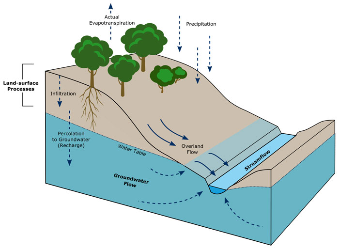
Figure 1: Terrestrial water cycle schematic showing processes and storages. Groundwater denotes water in aquifers. The watershed is everything that is not a stream or aquifer.
Two conceptual end-member model types: 1) process-driven and 2) data-driven are used in hydrology for representation of water cycle components and estimation of the water budget. Process–driven models are the ‘classic’ models of hydrology; they use physics– and empirically–based relationships of hydrologic processes. Process–driven modeling assumes that we know and understand the processes that occur within the water cycle. Data–driven models are deep learning (DL) and machine learning (ML) implementations. Data–driven approaches assume that we know the data and that the model can be trained to learn or represent the processes. Long Short–Term Memory (LSTM) networks are the DL formulation employed in this study.
APPROACH
Our goal is to integrate process–driven and data–driven techniques into a single water budget model of the terrestrial hydrologic cycle. The starting point is a process–driven, water balance model that was created and implemented for a completed commercial project; the configuration of this model is shown on Figure 2. The main limitation of this model is that it represents a complex water cycle environment in karst terrain that contains unknown flow connections through unmapped caves and conduits in the subsurface. This flow path uncertainty means that we do not know all physical processes operating across the study area and makes this site a candidate for implementation of a data–driven model.
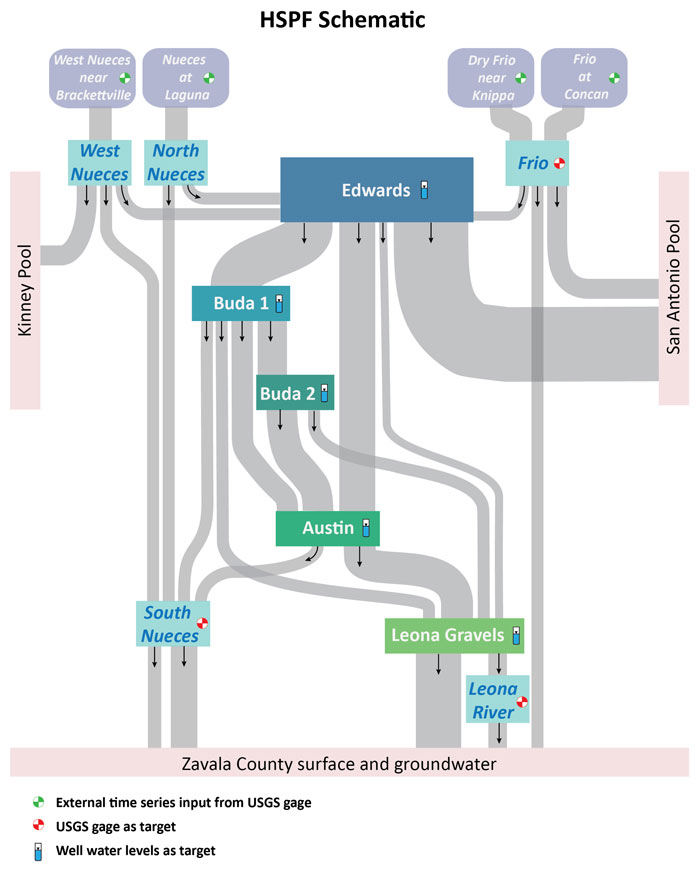
Figure 2: Existing process-based water budget model schematic. ‘HSPF’ is the process-based model used. In the integrated modeling approach, an LSTM network model represents or reproduces the data sets identified as ‘target’ locations. The process–based, HSPF model represents the movement of water along the gray pathways between targets and the volumes of water stored in the well water level target locations.
Figure 2 identifies the conceptual locations of the available data sets in the study area; ‘target’ locations correspond to data set locations. Integration of the existing process–driven approach with a data–driven approach involves training an LSTM model to reproduce these ‘target’ data sets. Then, the two models can be integrated so that the process–driven model provides water budget accounting for water movement and storage between data set locations. The use case for this type of integrated model is for historical and future conditions (i.e., periods without data sets).
ACCOMPLISHMENTS
- LSTM network model has been trained and tested. Its predictions provide a significant increase, from 3.7 to 7.0, in our aggregated ‘goodness-of-fit’ metric, which ranges from negative infinity to 8.0 with 8.0 being a ‘perfect’ fit. We were hoping for an increase of 2.0 to 3.0 (i.e., from 3.7 to 5.7–6.7).
- LSTM network model representation for the three USGS gage ‘target’ data sets in Figure 2 have been integrated to the process–based model.
- As part of LSTM network training, we realized that our stream gage data sets had significant quality issues. This is not surprising as the quantity of interest is continuous stream discharge at the gage location, and the observed or measured quantity is stream depth. Discharge is estimated from observed stream depth. We developed a standard error envelope estimation procedure for stream gage discharge data sets for use within iterative ensemble smoother approaches.